


This is a basic introduction of Proximal Policy Optimization (the best reinforcement learning algorithm in 2020) for machine learning folks like me who are not familiar with reinforcement learning.
Hung-yi Lee's lecture (in Chinese)
Proximal Policy Gradient (the paper)
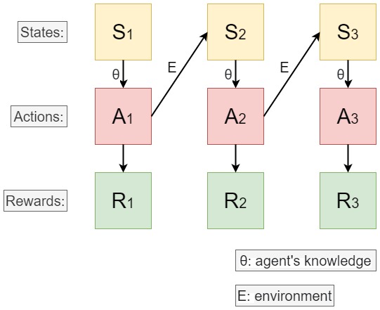
The problem definition of reinforcement learning was based on the interactions of the environment and the agent. As shown above, each state represent the observation made by the agent on the environment. Given each state, the agent will take an action based on its knowledge that maximize the future rewards. Together, the interaction will generate a sequence of states and actions. If we denote such sequence as $\tau$,
$$ \tau = \{ s_1, a_1, s_2, a_2, s_3, a_3 ... \} $$
we can write down the expected rewards of $\tau$ since $\tau$ is a random variable.
$$ \bar{R_{\theta}} = E_{\tau \sim p_\theta(\tau)} \big[ R(\tau) \big] = \sum_{\tau} R(\tau) p_{\theta}(\tau) ,\,\,\, R(\tau) = \sum_{i}^{T} r_t $$
In the case of deep reinforcement learning, $\theta$ is the neural network weights we want to adjust to maximize the expected rewards.
To optimize this expected rewards, we can take the derivative of it,
\begin{align} \nabla \bar{R_{\theta}} &= \sum_{\tau} R(\tau) \nabla p_{\theta}(\tau) \\ &= \sum_{\tau} R(\tau) p_{\theta}(\tau) \nabla \log p_{\theta}(\tau) \tag{$ \nabla \log f(x) = \frac{\log f(x)}{f(x)}$} \\ &= E_{\tau \sim p_\theta(\tau)} \big[ R(\tau) \nabla \log p_\theta(\tau) \big] \\ &\approx \frac{1}{N} \sum_{n=1}^{N} R(\tau^n) \nabla \log p_\theta(\tau^n) \\ &= \frac{1}{N} \sum_{n=1}^{N} \sum_{t=1}^{T_n} R(\tau^n) \nabla \log p_\theta(a_t^n | s_t^n) \tag{$ \nabla \log p_\theta(\tau^n) = \sum_{t=1}^{T_n} \nabla \log p_\theta(a_t^n | s_t^n) $}\\ \end{align}
and then adjust $\theta$ with gradient descent,
$$ \theta \leftarrow \theta + \eta \nabla \bar{R_{\theta}} $$
This is equivalent to maximizing the log likelihood of the action at each time step weighted by the rewards of a sequence. However, we also maximize the likelihood of the wrong actions, but under softmax, the action with a higher reward will always have a higher probability of emission in the ideal scenario. Another issue is that in practice, we won't be able to sample all actions; to eliminate the bias from the partial sampling, we can subtract a positive constant term $b$ to punish the low rewards action,
$$ \nabla \bar{R_{\theta}} \approx \frac{1}{N} \sum_{n=1}^{N} \sum_{t=1}^{T_n} (R(\tau^n) - b) \nabla \log p_\theta(a_t^n | s_t^n) $$
An alternative solution is to replace the reward term with a critic network,
$$ \nabla \bar{R_{\theta}} \approx \frac{1}{N} \sum_{n=1}^{N} \sum_{t=1}^{T_n} A^{\theta}(s_t, a_t) \nabla \log p_\theta(a_t^n | s_t^n) $$
The optimization approach above is called on-policy optimization, but in practice, off-policy optimization was used because the number of passes required by gradient descent usually exceeds the number of sample data. In such setting, one would want to optimize $\theta$ based on the data previously sampled by another agent with weight $\theta_2$. This is the procedure:
1. sample data $D$ using agent with weight $\theta_2$
2. optimizing agent with weight $\theta$ using the data $D$ (multiple times)
3. sync up weights: $\theta_2 \leftarrow \theta$
Since $\theta$ and $\theta_2$ will create two different distributions, we need to use a technique called importance sampling to correct our expected rewards. An expected value under distribution $p$ can be rewritten using another distribution $q$,
$$ E_{x \sim p} [f(x)] = \int f(x) p(x) dx = \int f(x) \frac{p(x)}{q(x)} q(x) dx = E_{x \sim q} [f(x) \frac{p(x)}{q(x)}] $$
Look back at our policy gradient,
$$ \nabla \bar{R_{\theta}} = E_{(a_t, s_t) \sim p_\theta(\tau)} [A^{\theta}(s_t, a_t) \nabla \log p_\theta(a_t | s_t)] $$
If we rewrite the expected rewards for $\theta$ (the learner agent) using importance sampling from $\theta_2$ (the agent in the environment), we get,
\begin{align} \nabla \bar{R_{\theta}} &= E_{(a_t, s_t) \sim p_{\theta_2}(\tau)} [\frac{ p_{\theta_2}(a_t, s_t) }{ p_{\theta}(a_t, s_t) } A^{\theta_2}(s_t, a_t) \nabla \log p_\theta(a_t | s_t)] \\ &= E_{(a_t, s_t) \sim p_{\theta_2}(\tau)} [\frac{ p_{\theta_2}(a_t | s_t) }{ p_{\theta}(a_t | s_t) } A^{\theta_2}(s_t, a_t) \nabla \log p_\theta(a_t | s_t)] \tag{$p_{\theta}(s_t) = p_{\theta_2}(s_t)$}\\ \end{align}
After taking the integral of the above policy gradient, we get the new expected rewards in the importance sampling setting,
\begin{align} \bar{R_{\theta}} = E_{(a_t, s_t) \sim p_{\theta_2}(\tau)} [\frac{ p_{\theta_2}(a_t | s_t) }{ p_{\theta}(a_t | s_t) } A^{\theta_2}(s_t, a_t) ] \tag{ $ \nabla \log f(x) = \frac{\log f(x)}{f(x)}$ } \end{align}
We have shown that the addition of important sampling doesn't change the expected rewards,
$$ E_{x \sim p} [f(x)] = E_{x \sim q} [f(x) \frac{p(x)}{q(x)}] $$
However, the variance of rewards under these two settings are different,
$$ Var_{x \sim p} [f(x)] \neq Var_{x \sim q} [f(x) \frac{p(x)}{q(x)}] $$
In the vanilla setting is,
$$ Var_{x \sim p} [f(x)] = E_{x \sim p} [f(x)^2] - (E_{x \sim p} [f(x)])^2 \tag{definition of variance} $$
In the important sampling setting,
\begin{align} Var_{x \sim q} [f(x) \frac{p(x)}{q(x)}] &= E_{x \sim q} [(f(x) \frac{p(x)}{q(x)})^2] - (E_{x \sim q} [f(x) \frac{p(x)}{q(x)}])^2 \\ &= E_{x \sim p} [f(x)^2 \frac{p(x)}{q(x)}] - (E_{x \sim p} [f(x)])^2 \end{align}
When $p(x)$ is very different from $q(x)$, the effectiveness of the important sampling technique will be reduced. In practice, we want $p(x)$ to be closer to $q(x)$
To constraint the difference between $p(x)$ and $q(x)$, Proximal Policy Gradient adds a regularization term on top of importance sampling,
$$ \bar{R^{\theta}_{PPO}} = E_{(a_t, s_t) \sim p_{\theta_2}(\tau)} [\frac{ p_{\theta_2}(a_t | s_t) }{ p_{\theta}(a_t | s_t) } A^{\theta_2}(s_t, a_t) ] + \beta KL (\theta, \theta_2) $$
where $KL (\theta, \theta_2)$ is the KL-divergence of $ p_{\theta} (a_t \vert s_t) $ and $ p_{\theta_2} (a_t \vert s_t) $, and $\beta$ is a hyperparameter. Intuitively, when we build a new agent based on a previously trained agent, we don't want the new agent to be too much different from the starting point. This allows the algorithm to make finer but incremental update to our model. Alternatively, we cloud also use clipping with a hyperparamter $\epsilon$ to implement this idea,
$$ \bar{R^{\theta}_{PPO_2}} = E_{(a_t, s_t) \sim p_{\theta_2}(\tau)} [min( \frac{ p_{\theta_2}(a_t | s_t) }{ p_{\theta}(a_t | s_t) } A^{\theta_2}(s_t, a_t), \, clip(\frac{ p_{\theta_2}(a_t | s_t) }{ p_{\theta}(a_t | s_t) }, 1-\epsilon, 1+\epsilon) A^{\theta_2}(s_t, a_t), )] $$
When $A^{\theta_2}(s_t, a_t) > 0$ (good action), we set the upper limit of $\frac{ p_{\theta_2}(a_t \vert s_t) }{ p_{\theta}(a_t \vert s_t) }$ to be $ 1 + \epsilon $. When $A^{\theta_2}(s_t, a_t) < 0$ (bad action), we set the lower limit of $\frac{ p_{\theta_2}(a_t \vert s_t) }{ p_{\theta}(a_t \vert s_t) }$ to be $ 1 - \epsilon $.